Generating ATL03 photon classifications using ATL08 and YAPC

Plot ATL03 data with different classifications for a region over the Grand Mesa, CO region

• ATL08 Land and Vegetation Height product photon classification

• Experimental YAPC (Yet Another Photon Classification) photon-density-based classification

What is demonstrated

• The icesat2.atl03sp API is used to perform a SlideRule parallel subsetting request of the Grand Mesa region

• The earthdata.cmr API’s is used to find specific ATL03 granules corresponding to the Grand Mesa region

• The matplotlib package is used to plot the ATL03 data subset by SlideRule

import warnings
warnings.filterwarnings("ignore") # suppress warnings

import numpy as np
import matplotlib.pyplot as plt
from sliderule import sliderule, icesat2, earthdata

sliderule.init(verbose=True)

True

Intro

This notebook demonstrates how to use the SlideRule Icesat-2 API to retrieve ATL03 data with two different classifications, one based on the external ATL08-product classifications, designed to distinguish between vegetation and ground returns, and the other based on the experimental YAPC (Yet Another Photon Class) algorithm.

Retrieve ATL03 elevations with ATL08 classifications

define a polygon to encompass Grand Mesa, and pick an ATL03 granule that has good coverage over the top of the mesa. Note that this granule was captured at night, under clear-sky conditions. Other granules are unlikely to have results as clear s these.

%%time

# build sliderule parameters for ATL03 subsetting request
parms = {
    # processing parameters
    "srt": icesat2.SRT_LAND,
    "len": 20,
    "res": 20,
    # classification and checks
    # still return photon segments that fail checks
    "pass_invalid": True,
    # all photons
    "cnf": -2,
    # all land classification flags
    "atl08_class": ["atl08_noise", "atl08_ground", "atl08_canopy", "atl08_top_of_canopy", "atl08_unclassified"],
    # all photons
    "yapc": dict(knn=0, win_h=6, win_x=11, min_ph=4, score=0),
}

# ICESat-2 data release
release = '006'

# region of interest
poly = [
  {'lat': 39.34603060272382, 'lon': -108.40601489205419},
  {'lat': 39.32770853617356, 'lon': -107.68485163209928},
  {'lat': 38.770676045922684, 'lon': -107.71081820956682},
  {'lat': 38.788639821001155, 'lon': -108.42635020791396},
  {'lat': 39.34603060272382, 'lon': -108.40601489205419}
]

# time bounds for CMR query
time_start = '2019-11-14'
time_end = '2019-11-15'

# find granule for each region of interest
granules_list = earthdata.cmr(short_name='ATL03', polygon=poly, time_start=time_start, time_end=time_end, version=release)

# create geodataframe
gdf = sliderule.run("atl03x", parms, aoi=poly, resources=granules_list)

HTTP Request Error: HTTP Error 400: Bad Request
Using simplified polygon (for CMR request only!), 5 points using tolerance of 0.0001
Starting proxy for atl03x to process 1 resource(s) with 1 thread(s)
request <AppServer.78978> on ATL03_20191114034331_07370502_006_01.h5 generated dataframe [gt1l] with 66779 rows and 14 columns
request <AppServer.78978> on ATL03_20191114034331_07370502_006_01.h5 generated dataframe [gt2l] with 66801 rows and 14 columns
request <AppServer.78978> on ATL03_20191114034331_07370502_006_01.h5 generated dataframe [gt3l] with 63781 rows and 14 columns
request <AppServer.78978> on ATL03_20191114034331_07370502_006_01.h5 generated dataframe [gt2r] with 207158 rows and 14 columns
request <AppServer.78978> on ATL03_20191114034331_07370502_006_01.h5 generated dataframe [gt3r] with 255932 rows and 14 columns
request <AppServer.78978> on ATL03_20191114034331_07370502_006_01.h5 generated dataframe [gt1r] with 265252 rows and 14 columns
Successfully completed processing resource [1 out of 1]: ATL03_20191114034331_07370502_006_01.h5
Writing arrow file: /tmp/tmp1t6r6veh
Closing arrow file: /tmp/tmp1t6r6veh

CPU times: user 1.47 s, sys: 359 ms, total: 1.83 s
Wall time: 23.1 s

gdf

	region	gt	spacecraft_velocity	solar_elevation	yapc_score	rgt	ph_index	height	atl08_class	spot	x_atc	y_atc	srcid	cycle	atl03_cnf	background_rate	quality_ph	geometry
time_ns
2019-11-14 03:46:35.872218112	2	50	7113.586426	-44.078053	239	737	1075952	1507.619995	1	2	4.314530e+06	-3158.350098	0	5	4	5359.785645	0	POINT (-108.04141 38.77892)
2019-11-14 03:46:35.872218112	2	50	7113.586426	-44.078053	236	737	1075953	1507.708496	1	2	4.314530e+06	-3158.349365	0	5	4	5359.785645	0	POINT (-108.04141 38.77892)
2019-11-14 03:46:35.872317952	2	50	7113.586426	-44.078053	236	737	1075954	1507.787231	1	2	4.314531e+06	-3158.351807	0	5	4	5359.785645	0	POINT (-108.04141 38.77893)
2019-11-14 03:46:35.872317952	2	50	7113.586426	-44.078053	231	737	1075955	1508.115601	1	2	4.314531e+06	-3158.349365	0	5	4	5359.785645	0	POINT (-108.04141 38.77893)
2019-11-14 03:46:35.872418048	2	50	7113.586426	-44.078053	235	737	1075956	1508.048218	1	2	4.314532e+06	-3158.352783	0	5	4	5359.785645	0	POINT (-108.04141 38.77893)
...	...	...	...	...	...	...	...	...	...	...	...	...	...	...	...	...	...	...
2019-11-14 03:46:44.991418368	2	20	7113.345215	-43.875050	122	737	4680202	1551.664429	1	5	4.376748e+06	3145.825928	5	5	4	21039.835938	0	POINT (-108.18256 39.33137)
2019-11-14 03:46:44.991418368	2	20	7113.345215	-43.875050	116	737	4680203	1552.543823	0	5	4.376748e+06	3145.820068	5	5	4	21039.835938	0	POINT (-108.18256 39.33137)
2019-11-14 03:46:44.991418368	2	20	7113.345215	-43.875050	69	737	4680204	1547.385010	0	5	4.376748e+06	3145.854004	5	5	4	21039.835938	0	POINT (-108.18256 39.33137)
2019-11-14 03:46:44.991418368	2	20	7113.345215	-43.875050	128	737	4680205	1549.545044	0	5	4.376748e+06	3145.839844	5	5	4	21039.835938	0	POINT (-108.18256 39.33137)
2019-11-14 03:46:44.991418368	2	20	7113.345215	-43.875050	122	737	4680206	1551.820801	1	5	4.376748e+06	3145.824707	5	5	4	21039.835938	0	POINT (-108.18256 39.33137)

925703 rows × 18 columns

Reduce GeoDataFrame to plot a single beam

• Convert coordinate reference system to compound projection

gdf.keys()

Index(['region', 'gt', 'spacecraft_velocity', 'solar_elevation', 'yapc_score',
       'rgt', 'ph_index', 'height', 'atl08_class', 'spot', 'x_atc', 'y_atc',
       'srcid', 'cycle', 'atl03_cnf', 'background_rate', 'quality_ph',
       'geometry'],
      dtype='object')

def reduce_dataframe(gdf, RGT=None, GT=None, spot=None, cycle=None, crs=4326):
    D3 = gdf.to_crs(crs) # convert coordinate reference system
    if RGT is not None:
        D3 = D3[D3["rgt"] == RGT]
    if GT is not None:
        D3 = D3[D3["gt"] == GT]
    if spot is not None:
        D3 = D3[D3["spot"] == spot]
    if cycle is not None:
        D3 = D3[D3["cycle"] == cycle]
    return D3

project_srs = "EPSG:26912+EPSG:5703"
D3 = reduce_dataframe(gdf, RGT=737, spot=1, crs=project_srs)

Inspect Coordinate Reference System

D3.crs

<Compound CRS: EPSG:26912+EPSG:5703>
Name: NAD83 / UTM zone 12N + NAVD88 height
Axis Info [cartesian|vertical]:
- E[east]: Easting (metre)
- N[north]: Northing (metre)
- H[up]: Gravity-related height (metre)
Area of Use:
- undefined
Datum: North American Datum 1983
- Ellipsoid: GRS 1980
- Prime Meridian: Greenwich
Sub CRS:
- NAD83 / UTM zone 12N
- NAVD88 height

Plot the ATL08 classifications

plt.figure(figsize=[8,6])

colors={0:['gray', 'noise'],
        4:['gray','unclassified'],
        2:['green','canopy'],
        3:['lime', 'canopy_top'],
        1:['brown', 'ground']}
d0=np.min(D3['x_atc'])
for class_val, color_name in colors.items():
    ii=D3['atl08_class']==class_val
    plt.plot(D3['x_atc'][ii]-d0, D3['height'][ii],'o',
         markersize=1, color=color_name[0], label=color_name[1])
hl=plt.legend(loc=3, frameon=False, markerscale=5)
plt.gca().set_xlim([25000, 30000])
plt.gca().set_ylim([3050, 3300])

plt.ylabel('height, m')
plt.xlabel('$x_{ATC}$, m');

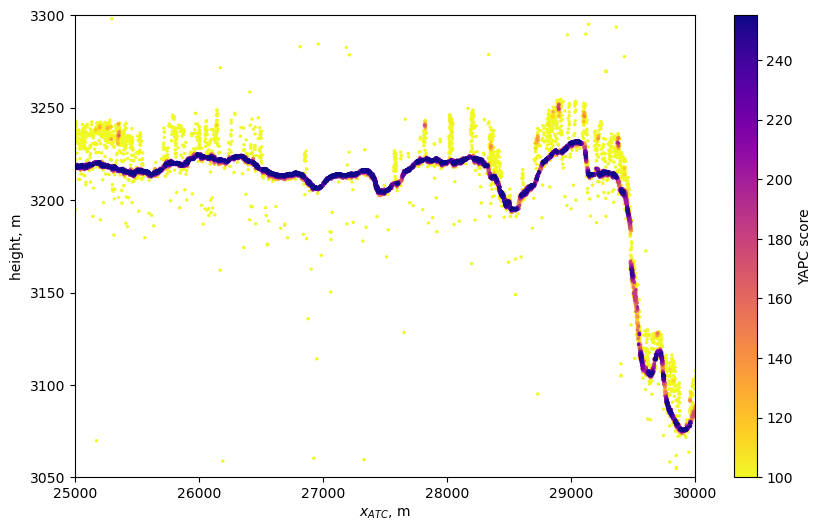
Plot the YAPC classifications

plt.figure(figsize=[10,6])

d0=np.min(D3['x_atc'])
ii=np.argsort(D3['yapc_score'])
plt.scatter(D3['x_atc'][ii]-d0,
    D3['height'][ii],2, c=D3['yapc_score'][ii],
    vmin=100, vmax=255, cmap='plasma_r')
plt.colorbar(label='YAPC score')
plt.gca().set_xlim([25000, 30000])
plt.gca().set_ylim([3050, 3300])

plt.ylabel('height, m')
plt.xlabel('$x_{ATC}$, m');