Sampling the ArcticDEM Mosaic

Purpose

Demonstrate how to sample the ArcticDEM at generated ATL06-SR points

Import Packages

[1]:

import matplotlib.pyplot as plt
import matplotlib
import sliderule
from sliderule import icesat2

Initialize SlideRule Python Client

[2]:

sliderule.init(verbose=True)

[2]:

True

Make Processing Request to SlideRule

ATL06-SR request includes the samples parameter to specify that ArcticDEM Mosiac dataset should be sampled at each generated ATL06 elevation.

[3]:

resource = "ATL03_20190314093716_11600203_005_01.h5"
region = sliderule.toregion("dicksonfjord.geojson")
parms = { "poly": region['poly'],
          "cnf": "atl03_high",
          "ats": 5.0,
          "cnt": 5,
          "len": 20.0,
          "res": 10.0,
          "samples": {"mosaic": {"asset": "arcticdem-mosaic", "radius": 10.0, "zonal_stats": True}} }
gdf = icesat2.atl06p(parms, resources=[resource])

proxy request <AppServer.78961> querying resources for mosaic
Starting proxy for atl06 to process 1 resource(s) with 1 thread(s)
request <AppServer.62913> processing initialized on ATL03_20190314093716_11600203_005_01.h5 ...
request <AppServer.62913> processing of ATL03_20190314093716_11600203_005_01.h5 complete (162852/1626/0)
request <AppServer.62913> processing complete (1696/1/1696/0)
Successfully completed processing resource [1 out of 1]: ATL03_20190314093716_11600203_005_01.h5

Display GeoDataFrame

Notice the columns that start with “mosaic”

[4]:

gdf

[4]:

	rgt	n_fit_photons	gt	y_atc	h_mean	x_atc	spot	region	h_sigma	rms_misfit	...	mosaic.median	mosaic.file_id	mosaic.value	mosaic.flags	mosaic.stdev	mosaic.max	mosaic.mad	mosaic.time	mosaic.count	mosaic.min
time
2019-03-14 09:40:46.291445504	1160	15	10	4678.975098	594.468321	8121554.0	1	3	0.187902	0.263953	...	584.289062	0	584.289062	0	4.606139	592.898438	3.984568	1.358109e+09	81	576.406250
2019-03-14 09:40:46.292858624	1160	27	10	4678.930664	595.268325	8121564.0	1	3	0.059746	0.269889	...	592.257812	0	592.562500	0	3.477136	596.804688	2.955249	1.358109e+09	81	583.507812
2019-03-14 09:40:46.294273792	1160	12	10	4678.869141	595.776378	8121574.0	1	3	0.328370	0.268849	...	596.843750	0	596.875000	0	2.326261	602.914062	1.928062	1.358109e+09	81	593.132812
2019-03-14 09:40:46.295686400	1160	9	10	4678.799805	605.299322	8121584.0	1	3	0.104096	0.174862	...	600.414062	0	600.414062	0	2.801560	606.117188	2.440825	1.358109e+09	81	596.296875
2019-03-14 09:40:46.297094912	1160	33	10	4678.792480	606.692014	8121594.0	1	3	0.162495	0.927663	...	605.265625	0	605.125000	0	2.346747	608.570312	2.013160	1.358109e+09	81	599.804688
...	...	...	...	...	...	...	...	...	...	...	...	...	...	...	...	...	...	...	...	...	...
2019-03-14 09:40:48.353273600	1160	27	20	4581.452148	1497.294367	8133741.0	2	3	0.053913	0.280013	...	1494.429688	0	1494.398438	0	0.497044	1495.468750	0.418148	1.358109e+09	81	1493.515625
2019-03-14 09:40:48.354683648	1160	15	20	4581.416016	1497.036678	8133751.0	2	3	0.114113	0.330651	...	1494.156250	0	1494.218750	0	0.559426	1495.273438	0.459164	1.358109e+09	81	1492.945312
2019-03-14 09:40:48.356088576	1160	8	20	4581.380371	1496.055088	8133761.0	2	3	0.046961	0.132604	...	1493.507812	0	1493.546875	0	0.750541	1494.906250	0.633445	1.358109e+09	81	1491.921875
2019-03-14 09:40:48.357494784	1160	16	20	4581.345703	1494.952556	8133771.0	2	3	0.032820	0.124317	...	1492.648438	0	1492.648438	0	0.844155	1494.187500	0.711853	1.358109e+09	81	1490.906250
2019-03-14 09:40:48.358897920	1160	19	20	4581.309082	1494.040127	8133781.0	2	3	0.028111	0.117033	...	1491.515625	0	1491.367188	0	0.878481	1493.062500	0.747692	1.358109e+09	81	1489.742188

1696 rows × 27 columns

Print Out File Directory

When a GeoDataFrame includes samples from rasters, each sample value has a file id that is used to look up the file name of the source raster for that value.

[5]:

gdf.attrs['file_directory']

[5]:

{0: '/vsis3/pgc-opendata-dems/arcticdem/mosaics/v4.1/2m_dem_tiles.vrt'}

Demonstrate How To Access Source Raster Filename for Entry in GeoDataFrame

[6]:

filedir = gdf.attrs['file_directory']
filedir[gdf['mosaic.file_id'].iloc[0]]

[6]:

'/vsis3/pgc-opendata-dems/arcticdem/mosaics/v4.1/2m_dem_tiles.vrt'

Difference the Sampled Value from ArcticDEM with SlideRule ATL06-SR

[7]:

gdf["value_delta"] = gdf["h_mean"] - gdf["mosaic.value"]
gdf["value_delta"].describe()

[7]:

count    1696.000000
mean        1.130969
std         2.161111
min       -27.810532
25%         0.264682
50%         1.273614
75%         2.154959
max        14.924781
Name: value_delta, dtype: float64

Difference the Zonal Statistic Mean from ArcticDEM with SlideRule ATL06-SR

[8]:

gdf["mean_delta"] = gdf["h_mean"] - gdf["mosaic.mean"]
gdf["mean_delta"].describe()

[8]:

count    1696.000000
mean        1.141126
std         2.167836
min       -28.240605
25%         0.253310
50%         1.283650
75%         2.165268
max        15.173141
Name: mean_delta, dtype: float64

Difference the Zonal Statistic Mdeian from ArcticDEM with SlideRule ATL06-SR

[9]:

gdf["median_delta"] = gdf["h_mean"] - gdf["mosaic.median"]
gdf["median_delta"].describe()

[9]:

count    1696.000000
mean        1.139339
std         2.162717
min       -27.716782
25%         0.253184
50%         1.277012
75%         2.154026
max        14.924781
Name: median_delta, dtype: float64

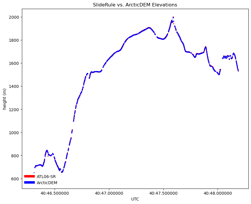
Plot the Different ArcticDEM Values against the SlideRule ATL06-SR Values

[10]:

# Setup Plot
fig,ax = plt.subplots(num=None, figsize=(10, 8))
fig.set_facecolor('white')
fig.canvas.header_visible = False
ax.set_title("SlideRule vs. ArcticDEM Elevations")
ax.set_xlabel('UTC')
ax.set_ylabel('height (m)')
legend_elements = []

# Plot SlideRule ATL06 Elevations
df = gdf[(gdf['rgt'] == 1160) & (gdf['gt'] == 10) & (gdf['cycle'] == 2)]
sc1 = ax.scatter(df.index.values, df["h_mean"].values, c='red', s=2.5)
legend_elements.append(matplotlib.lines.Line2D([0], [0], color='red', lw=6, label='ATL06-SR'))

# Plot ArcticDEM Elevations
sc2 = ax.scatter(df.index.values, df["mosaic.value"].values, c='blue', s=2.5)
legend_elements.append(matplotlib.lines.Line2D([0], [0], color='blue', lw=6, label='ArcticDEM'))

# Display Legend
lgd = ax.legend(handles=legend_elements, loc=3, frameon=True)
lgd.get_frame().set_alpha(1.0)
lgd.get_frame().set_edgecolor('white')

# Show Plot
plt.show()

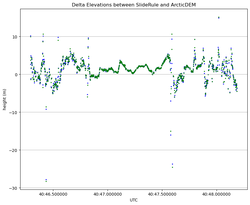
../_images/assets_arcticdem_mosaic_20_0.png

Plot the Sampled Value and Zonal Statistic Mean Deltas to SlideRule ATL06-SR Values

[11]:

# Setup Plot
fig,ax = plt.subplots(num=None, figsize=(10, 8))
fig.set_facecolor('white')
fig.canvas.header_visible = False
ax.set_title("Delta Elevations between SlideRule and ArcticDEM")
ax.set_xlabel('UTC')
ax.set_ylabel('height (m)')
ax.yaxis.grid(True)

# Plot Deltas
df1 = gdf[(gdf['rgt'] == 1160) & (gdf['gt'] == 10) & (gdf['cycle'] == 2)]
sc1 = ax.scatter(df1.index.values, df1["value_delta"].values, c='blue', s=2.5)

# Plot Deltas
df2 = gdf[(gdf['rgt'] == 1160) & (gdf['gt'] == 10) & (gdf['cycle'] == 2)]
sc2 = ax.scatter(df2.index.values, df2["mean_delta"].values, c='green', s=2.5)

# Show Plot
plt.show()

../_images/assets_arcticdem_mosaic_22_0.png

[ ]: